Note
Go to the end to download the full example code.
Adapative Cruise Control with Input Constrained Control Barrier Function#
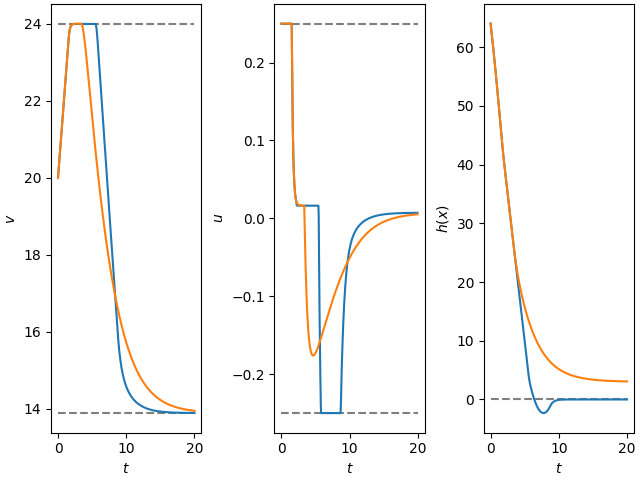
This example demonstrates the use of Input Constrained Control Barrier Functions (ICCBFs) in the context of the Adaptive Cruise Control (ACC) problem, taken from [1]. The ACC problem is a classic control problem where a vehicle is tasked with maintaining a desired velocity while keeping a safe distance from the vehicle in front. This safety constraint is enforced using a ICCBF, which is a class of CBFs that can handle the case where the control input is constrained in its norm.
Defining the state \(x = \begin{bmatrix} d & v \end{bmatrix}^\top\), the dynamics of the vehicle are
with \(u \in [-0.25, 0.25]\) being the control input. Safety is described by the safe set
To control such dynamics, in this example we implement two controllers: a CLF-CBF-QP that does not consider input constraints, and the ICCBF-QP that does.
References#
import sys

if sys.version_info >= (3, 10):
    from typing import TypeAlias
else:
    from typing_extensions import TypeAlias

from typing import Any, Callable, Optional

import casadi as cs
import gymnasium as gym
import numpy as np
import numpy.typing as npt
from gymnasium.spaces import Box
from scipy.integrate import solve_ivp

from mpcrl.util.control import cbf, iccbf
from mpcrl.util.math import SymOrNumType, clip, lie_derivative

SOLVER = "qrqp"
OPTS = {
    "error_on_fail": True,
    "print_time": False,
    "verbose": False,
    "print_info": False,
    "print_iter": False,
    "print_header": False,
}
Defining the environment#
As commonly done in other examples, we first define the environment via gymnasium.
The environment also exposes two additional methods, AccEnv.dynamics and
AccEnv.h, to quickly compute the dynamics and the safety constraint,
respectively.
ObsType: TypeAlias = npt.NDArray[np.floating]
ActType: TypeAlias = npt.NDArray[np.floating]


class AccEnv(gym.Env[ObsType, ActType]):
    """Adaptive Cruise Control environment."""

    ns = 2
    na = 1
    # params
    m = 1650.0
    f0 = 0.1
    f1 = 5.0
    f2 = 0.25
    v0 = 13.89
    vmax = 24.0
    g = 9.81
    umax = 0.25

    def __init__(self, sampling_time: float) -> None:
        super().__init__()
        self.observation_space = Box(-np.inf, np.inf, (self.ns,), np.float64)
        self.action_space = Box(-self.umax, self.umax, (self.na,), np.float64)
        self.dt = sampling_time
        self.x: ObsType

        x = cs.SX.sym("x", self.ns)
        friction = self.f0 + self.f1 * x[1] + self.f2 * x[1] ** 2
        f = cs.vertcat(self.v0 - x[1], -friction / self.m)
        g = cs.vertcat(0, self.g)
        self.dynamics_components = cs.Function("dyn", (x,), (f, g), ("x",), ("f", "g"))

    def reset(
        self, *, seed: Optional[int] = None, options: Optional[dict[str, Any]] = None
    ) -> tuple[ObsType, dict[str, Any]]:
        super().reset(seed=seed, options=options)
        self.x = np.asarray([100, 20])
        assert self.observation_space.contains(self.x), f"invalid reset state {self.x}"
        return self.x, {}

    def step(
        self, action: npt.ArrayLike
    ) -> tuple[ObsType, float, bool, bool, dict[str, Any]]:
        x = self.x
        u = np.asarray(action).reshape(self.na)
        assert self.action_space.contains(u), f"invalid action {u}"

        sol = solve_ivp(
            lambda _, x: self.dynamics(x, u).toarray().flatten(),
            (0, self.dt),
            x,
            method="DOP853",
        )
        assert sol.success, f"integration failed: {sol.message}"

        x_new = sol.y[:, -1]
        assert self.observation_space.contains(x_new), f"invalid new state {x_new}"
        self.x = x_new
        return x_new, np.nan, False, False, {}

    def dynamics(self, x: SymOrNumType, u: SymOrNumType) -> SymOrNumType:
        """Computes the dynamics of the system."""
        f, g = self.dynamics_components(x)
        return f + g @ u

    def h(self, y: SymOrNumType) -> SymOrNumType:
        """Safety constraint."""
        return y[0] - 1.8 * y[1]
Controllers#
Now we implement two different types of controller. The first one is based on the CLF-CBF-QP method, which uses a Quadratic Program (QP) to find the control input that minimizes a cost function while satisfying the CLF and CBF constraints. It does not consider input constraints, so we need to clip the optimal action before pasing it to the environment. The second controller is based on the ICCBF-QP method, which does consider input constraints.
CLF-CBF-QP controller#
The following function creates the CLF-CBF-QP controller. We provide the method
mpcrl.util.control.cbf to quickly impose continuous-time high-order CBF
constraints.
def create_clf_cbf_qp(env: AccEnv) -> Callable[[ObsType], ActType]:
    """Returns the control law based on the CLF-CBF-QP method."""
    x = cs.MX.sym("x", env.ns)
    u = cs.MX.sym("u", env.na)
    delta = cs.MX.sym("delta")
    f, g = env.dynamics_components(x)

    V = (x[1] - env.vmax) ** 2
    LfV, LgV = lie_derivative(V, x, f), lie_derivative(V, x, g)
    clf_cnstr = LfV + LgV * u + 10 * V - delta

    cbf_cnstr = cbf(env.h, x, u, lambda x_, u_: env.dynamics(x_, u_), [lambda y: 2 * y])

    qp = {
        "x": cs.vertcat(u, delta),
        "p": x,
        "f": 0.5 * cs.sumsqr(u) + 0.1 * delta,
        "g": cs.vertcat(clf_cnstr, -cbf_cnstr),
    }
    lbx = np.append(np.full(env.na, -np.inf), 0)
    ubx = np.full(env.na + 1, np.inf)
    solver = cs.qpsol("solver_clf_cbf_qp", SOLVER, qp, OPTS)
    res = solver(p=x, lbx=lbx, ubx=ubx, lbg=-np.inf, ubg=0)
    u_clf_cbf_qp = clip(res["x"][: env.na], env.action_space.low, env.action_space.high)
    return cs.Function("clf_cbf_qp", [x], [u_clf_cbf_qp], ["x"], ["u"])
ICCBF-QP controller#
Here instead we define the ICCBF-QP controller. We provide the method
mpcrl.util.control.iccbf to create continuous-time ICCBFs.
def create_iccbf_qp(env: AccEnv) -> cs.Function:
    """Returns the control law based on the ICCLF-QP method."""
    x = cs.MX.sym("x", env.ns)
    u = cs.MX.sym("u", env.na)
    f, g = env.dynamics_components(x)

    V = (x[1] - env.vmax) ** 2
    LfV, LgV = lie_derivative(V, x, f), lie_derivative(V, x, g)
    u_des = -(10 * V + LfV) / LgV

    alphas = [lambda y: 4 * y, lambda y: 7 * cs.sqrt(y), lambda y: 2 * y]
    iccbf_cnstr = iccbf(
        env.h, x, u, env.dynamics_components, alphas, norm=1, bound=env.umax
    )

    qp = {"x": u, "p": x, "f": 0.5 * cs.sumsqr(u - u_des), "g": iccbf_cnstr}
    solver = cs.qpsol("solver_iccbf_qp", SOLVER, qp, OPTS)
    res = solver(p=x, lbx=env.action_space.low, ubx=env.action_space.high, lbg=0)
    u_iccbf_qp = res["x"]
    return cs.Function("iccbf_qp", [x], [u_iccbf_qp], ["x"], ["u"])
Simulation and Plots#
first, create a short function that simulates a given controller
def simulate_controller(
    env: AccEnv, ctrl: cs.Function, timesteps: int
) -> tuple[npt.ArrayLike, npt.ArrayLike]:
    """Simulates the environment with the given controller."""
    state, _ = env.reset()
    S, A = [state], []
    for _ in range(timesteps):
        action = ctrl(state)
        state, _, _, _, _ = env.step(action)
        S.append(state)
        A.append(action)
    return np.squeeze(S), np.squeeze(A)


# We can now simulate the two controllers and plot the results as in the original paper.


if __name__ == "__main__":
    # create the env
    Tfin = 20
    timesteps = 500
    env = AccEnv(Tfin / timesteps)

    # simulate the CLF-CBF-QP controller (num. 1)
    clf_cbf_qp_ctrl = create_clf_cbf_qp(env)
    S1, A1 = simulate_controller(env, clf_cbf_qp_ctrl, timesteps)

    # simulate the ICCBF-QP controller (num. 2)
    iccbf_qp_ctrl = create_iccbf_qp(env)
    S2, A2 = simulate_controller(env, iccbf_qp_ctrl, timesteps)

    # plot the results
    import matplotlib.pyplot as plt

    fig, axs = plt.subplots(1, 3, constrained_layout=True, sharex=True)

    T = np.arange(timesteps + 1) * env.dt
    S1, A1 = np.squeeze(S1), np.squeeze(A1)
    H1 = env.h(S1.T)
    S2, A2 = np.squeeze(S2), np.squeeze(A2)
    H2 = env.h(S2.T)

    limit_kw = {"xmin": T[0], "xmax": T[-1], "ls": "--", "color": "k", "alpha": 0.5}
    axs[0].hlines([env.v0, env.vmax], **limit_kw)
    axs[0].plot(T, S1[:, 1])
    axs[0].plot(T, S2[:, 1])
    axs[1].hlines([env.action_space.low, env.action_space.high], **limit_kw)
    axs[1].plot(T[:-1], A1)
    axs[1].plot(T[:-1], A2)
    axs[2].hlines(0.0, **limit_kw)
    axs[2].plot(T, H1)
    axs[2].plot(T, H2)

    for ax in axs:
        ax.set_xlabel("$t$")
    axs[0].set_ylabel("$v$")
    axs[1].set_ylabel("$u$")
    axs[2].set_ylabel("$h(x)$")

    plt.show()
Total running time of the script: (0 minutes 1.254 seconds)
Estimated memory usage: 192 MB